<?xml version="1.0" encoding="utf-8"?><feed xmlns="http://www.w3.org/2005/Atom" ><generator uri="https://jekyllrb.com/" version="3.10.0">Jekyll</generator><link href="https://ianchen3.github.io/feed.xml" rel="self" type="application/atom+xml" /><link href="https://ianchen3.github.io/" rel="alternate" type="text/html" /><updated>2026-08-24T05:19:44+00:00</updated><id>https://ianchen3.github.io/feed.xml</id><title type="html">Ian Chen</title><subtitle>Homepage</subtitle><author><name>Ian Chen</name><email>ianchen3@illinois.edu</email></author><entry><title type="html">2026 July Mindbenders</title><link href="https://ianchen3.github.io/posts/2026/07/mb" rel="alternate" type="text/html" title="2026 July Mindbenders" /><published>2026-07-16T00:00:00+00:00</published><updated>2026-07-16T00:00:00+00:00</updated><id>https://ianchen3.github.io/posts/2026/07/momath</id><content type="html" xml:base="https://ianchen3.github.io/posts/2026/07/mb"><![CDATA[<p>If you roll six dice, you could get the same number on every die, or (in contrast) all different numbers.
What is the probability of getting exactly four distinct numbers?
<a href="https://momath.org/mindbenders/">source</a>.</p>

<h1 id="guestimations-and-heuristics">Guestimations and Heuristics</h1>

<p>For a first approximation, we can look at the mean and variance of the number of distinct numbers.
Letting \(X_i\) be the event that we have at least one \(i\), \(X\) the number of distinct, then by linearity of expectation,</p>

\[\textbf{E}(X) = 6(1 - (5/6)^6) \approx 3.99\]

<p>which is very close to \(4\).
Hmm… this seems intentionally designed.
Let’s now calculate the variance: for \(i \ne j\), then</p>

\[\begin{align*}
  \textbf{E}(X_i X_j) &amp; = 1 - 2 \textbf{P}( \text{no dice on } i ) + \textbf{P}( \text{no dice on either } i, j ) \\
                      &amp; = 1 - 2 (5/6)^6 + (4/6)^6
\end{align*}\]

<p>so that</p>

\[\textbf{Var}(X) = \sum_{i=1}^6 \textbf{E}(X^2_i) + \sum_{i \ne j} \textbf{E}(X_i X_j) - \textbf{E}(X)^2 \approx 0.61\]

<p>A simple Chebyschev inqualities gives us that</p>

\[\textbf{P}(X = 4) = 1 - \textbf{P}( |{X - \textbf{E}(X)}| \ge (\textbf{E}(X) - 3) ) \ge 1 -  \frac{\textbf{Var}(X)}{(\textbf{E}(X) - 3)^2} = 0.382\]

<p>and a normal approximation gives us</p>

\[\Phi\left( \frac{4.5 - \textbf{E}(X)}{\sqrt{\textbf{Var}(X)}} \right) - \Phi\left( \frac{3.5 - \textbf{E}(X)}{\sqrt{\textbf{Var}(X)}} \right) \approx 0.48\]

<p>As an aside, this ratio \((1 - (1 - 1/n)^n ) \to 1 - \frac{1}{e} \approx 0.63\) is related to how hash maps set their maximum load.
If we hash \(n\) elements into \(n\) buckets uniformly, this is our expected occupancy!</p>

<h1 id="solutions">Solutions</h1>

<h2 id="some-code">Some code</h2>

<p>Not the most efficient, but some pretty clean usage brute-force calculation via the Python standard library.</p>

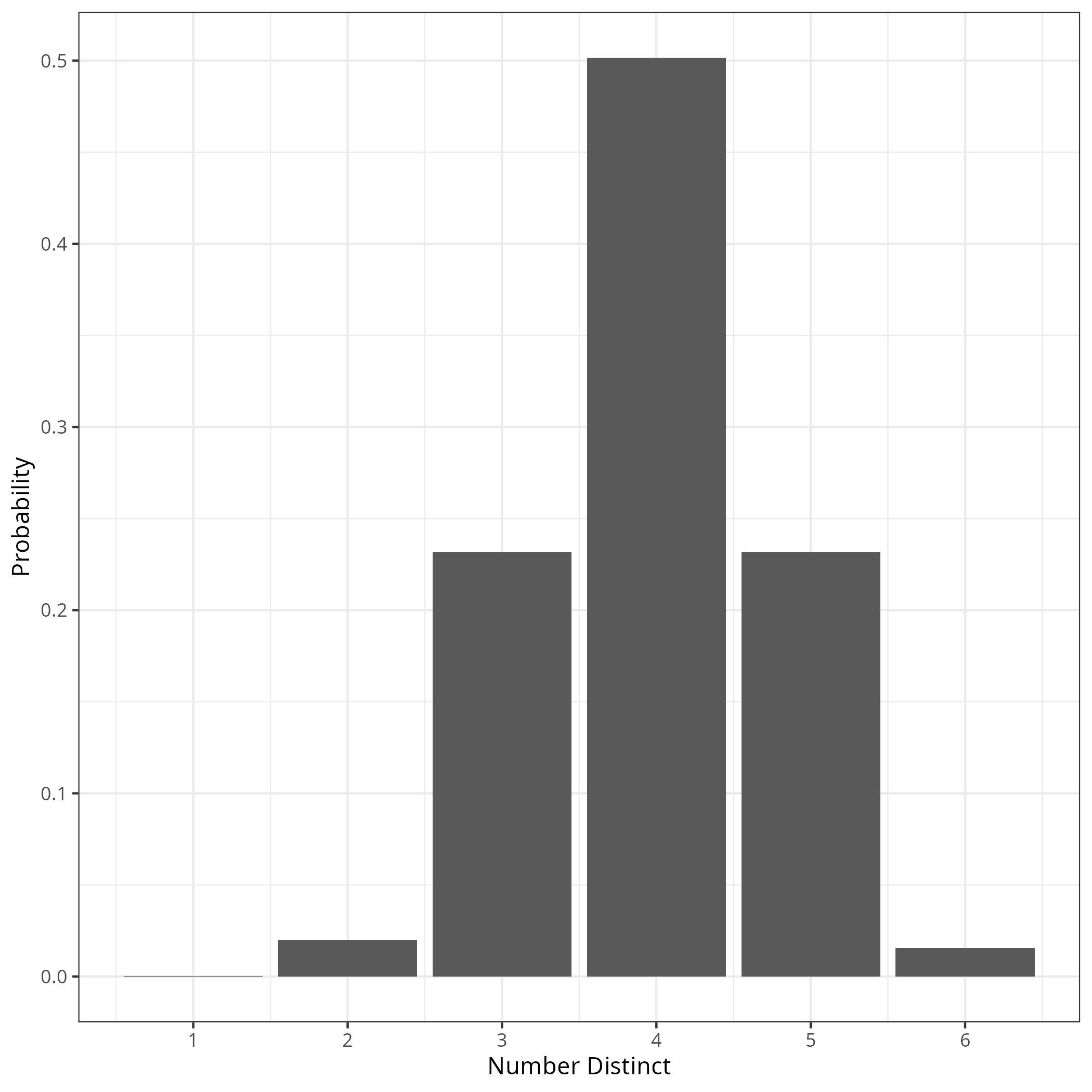
<div class="language-python highlighter-rouge"><div class="highlight"><pre class="highlight"><code><span class="o">&gt;</span> <span class="n">Counter</span><span class="p">(</span><span class="nb">len</span><span class="p">(</span><span class="nb">set</span><span class="p">(</span><span class="n">x</span><span class="p">))</span> <span class="k">for</span> <span class="n">x</span> <span class="ow">in</span> <span class="n">it</span><span class="p">.</span><span class="n">product</span><span class="p">(</span><span class="nb">range</span><span class="p">(</span><span class="mi">6</span><span class="p">),</span> <span class="n">repeat</span><span class="o">=</span><span class="mi">6</span><span class="p">))</span>
<span class="n">Counter</span><span class="p">({</span><span class="mi">4</span><span class="p">:</span> <span class="mi">23400</span><span class="p">,</span> <span class="mi">3</span><span class="p">:</span> <span class="mi">10800</span><span class="p">,</span> <span class="mi">5</span><span class="p">:</span> <span class="mi">10800</span><span class="p">,</span> <span class="mi">2</span><span class="p">:</span> <span class="mi">930</span><span class="p">,</span> <span class="mi">6</span><span class="p">:</span> <span class="mi">720</span><span class="p">,</span> <span class="mi">1</span><span class="p">:</span> <span class="mi">6</span><span class="p">})</span>
</code></pre></div></div>

<div style="text-align: center;">
  <img src="/files/posts/07-16-mb/histogram.png" />
</div>

<h2 id="combinatorics">Combinatorics</h2>

<p>There are \(6^6 = 46'656\) possible strings of 6 dice.
We want to derive an expression for \(c_k\), the number of ways for there to be exactly \(k\) distinct numbers in that string.</p>

<p>We first pick the \(k\) distinct numbers, with there being \(\binom{6}{k}\) different ways of doing so.
Then, we need to pick the histogram of counts for each of the \(k\) numbers.
For \(c_4\), then this is</p>

\[\binom{6}{4} \times \left(
    \frac{6!}{1! \cdot 1! \cdot 1! \cdot 3!} \times \frac{4!}{3! \cdot 1!} +
    \frac{6!}{1! \cdot 1! \cdot 2! \cdot 2!} \times \frac{4!}{2! \cdot 2!}
  \right) = 23'400\]

<p>And the answer is \(23'400 / 46'656 \approx 50.2\%\).
For some reason, \(c_3 = c_5\); seems like a coincidence.</p>

<p>There are many other ways to do this combinatorially, e.g. with generating functions or inclusion-exclusion.
These are besides the point here, but there are some more interesting approaches (many of which were in the pursuit of trying to find an intuitive reason for such a large probability mass)!</p>

<h2 id="dynamic-programming">Dynamic Programming</h2>

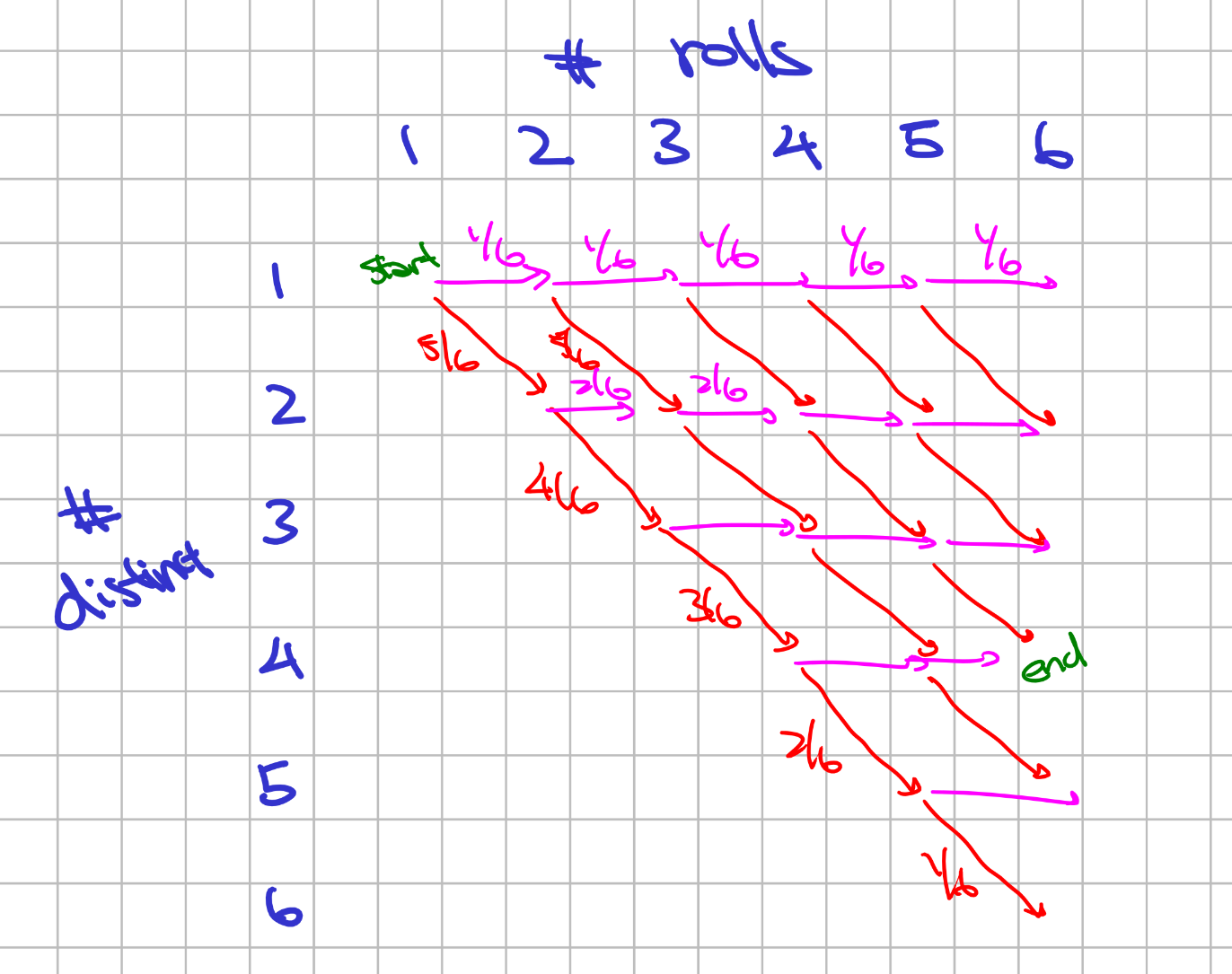
<p>Another approach that is maybe less error prone is to do some dynamic programming.
Let \(f(i, j)\) be the probability that we have \(i\) distinct numbers after \(j\) rolls.
Then, we get the recurrence</p>

\[f(i, j) =
  \begin{cases}
    1 &amp; i = j = 1 \\
    0 &amp; i &gt; j \\
    \frac{i}{6} \times f(i, j-1) + \frac{6-i}{6} f(i - 1, j) &amp; \text{otherwise}
  \end{cases}\]

<p>i.e. we sum up the cases where after a new roll, we get a distinct or not.</p>

<div style="text-align: center;">
  <img src="/files/posts/07-16-mb/dice-distinct.png" />
</div>

<p>Summing up each column gives a probability of exactly \(1\).
This also gives us a simpler closed form, namely, we just sum up all the paths!
Indeed,</p>

\[f(i, j) = \left( \prod_{k=7-i}^{5} \frac{k}{6} \right)
          \times 
          \left( \sum_{1 \le k_1 \le \ldots \le k_{j - i} \le i} \frac{ k_1 \cdot \ldots \cdot k_{j-i} }{6^{j-i}} \right)\]

<p>Calculating \(f(4, 6)\), the probability of getting \(4\) distinct numbers after \(6\) rolls, we have</p>

\[f(4, 6) = \frac{3}{6} \frac{4}{6} \frac{5}{6} \times \sum_{k_1=1}^4 \sum_{k_2=k_1}^4 \frac{k_1 \cdot k_2}{6^2}\]

<h2 id="hitting-times">Hitting Times</h2>

<p>Let us consider aa related problem: how many trials does it take until we get \(k\) distinct rolls.
The number of rolls until we get our first distinct follows \(\text{Geometric}(p = 1)\).
Our second distinct element follows \(\text{Geometric}(p = 1 - 1/6)\).
In general, to get the \(k\) -th distinct, it follows \(G_k = \text{Geometric}(p_k = \frac{7 - k}{6})\).
The expected number of rolls to get \(k = 1, \ldots, 6\) distinct elements are thus:</p>

\[1, 2.2, 3.7, 5.7, 8.7, 14.7\]

<p>But, if we recall from our introductory statistics classes, this feels a lot like the Poisson and Gamma duality.
The probability of counting \(\ge 4\) successes in \(6\) rolls is the same as it taking \(\le 6\) rolls to get the \(4\) -th success.</p>

<p>We can proceed in a similar path, deriving an analogous for the Gamma distribution.
In particular, let \(T_k = G_1 + \ldots + G_k\) be the rolls until we get the \(k\) -th distinct element.
Then, we want to calculate</p>

\[\textbf{Pr}(T_4 \le 6) - \textbf{Pr}( T_5 \le 6 )\]

<p>The full calculation is a bit annoying, and I have instead <a href="/files/posts/07-16-mb/duality.pdf">attached</a> it.
In short, probability generating functions are useful.</p>

<h2 id="embeddings">Embeddings</h2>

<p>An extremely powerful tool in stochastic processes, which I hope to learn more about, is to embed this discrete chain into some more general process.
Finally, we restrict our view of that more general process to the events that we care about.</p>

<p>This in general is known as Poissonification, and I first saw the idea with context of hashing in a UIUC theory seminar.
We suppose we throw \(m = \textbf{Poisson}(\lambda)\) die, and then condition on the event that \(m = 6\).
The really elegant result from this is that we avoid the negative correlation of the occupancy indicators \(X_i\).
In particular, if we look instead at the Multinomial distribution of the counts of each dice, then</p>

\[\begin{align*}
  &amp; \textbf{Pr}(\textbf{Multinomial}(m, (p_1, \ldots, p_6) = (n_1, \ldots, n_6); m \sim \textbf{Poisson}(\lambda)) \\
  &amp; = e^{- \lambda} \frac{\lambda^m}{m!} \times \frac{m!}{\prod_{i=1}^6 n_i!} \prod_{i=1}^6 p_i^{n_i} = \prod_{i=1}^6 e^{- \lambda p_i} \frac{(\lambda p_i)^{n_i}}{n_i!}
\end{align*}\]

<p>where we recognize each individual term in the product as the mass function for \(\textbf{Poisson}( \lambda p_i )\).
We not only avoid the negative correlation, but we get pure independence!
At this point, by conditioning on \(m\), we can do the <a href="/files/posts/07-16-mb/possonification.pdf">calculation</a> and get an answer.</p>

<p>In fact, if one remembers the construction of a Poisson process, then it should be clear why Possionification leads to this nice independence property.
Suppose we set a timer \(T \sim \textbf{Exponential}(\lambda / 6)\) independently for each of the \(6\) bins.
Then, a dice is rolled whenever a timer is fired, and the timer gets reset.</p>

<p>Here, the waiting time between rolls of the dice follow the minimum of \(6\) independent \(\textbf{Exponential}(\lambda / 6)\) timers, i.e. the gap between each of the each of the dice rolls follows \(\textbf{Exponential}(\lambda)\).
Thus, by the construction of Poisson process, then the number of dice rolls at a given time \(t\) follows \(\textbf{Poisson}( \lambda t )\).
Moreover, because exponential random variables are memoryless, then the increment between a dice rolling in each bin follows \(\textbf{Exponential}(\lambda / 6)\), and again by construction of Poisson, then the number of balls in a given bin follows \(\textbf{Poisson}(\lambda t / 6)\).</p>

<h1 id="a-long-thread">A Long Thread</h1>

<p>It feels like every stochastic process is just some variation on balls and bins.
Immediately, it is connected to hashing.
More generally, we can look at the waiting time, and other ways of embedding this into general chains, such as the Poisson process.
The DP is the simplest and hardest to make a mistake on (something about computing permutations just never goes right for me).
Then there are the more powerful generalizations, where looking at a continuous embedding (in the final clause) made the calculation much smoother than its discrete time analogs.
Generating functions, which I’ve hardly used before, were recurring, as the bridge to combine independent events.
While we have negatively correlated dependency structure, the right lens cast that away.</p>

<p>The goal of this multitude of approaches is to derive intuition for why we find such a large percentage of having 4 unique dice values.
My first instinct is to wave my hands with an exclaimation about the law of small numbers.
But this is a really good reminder about how common concentration really is – while these situations are rarely presented as a sum of independent events, the right view exposes it.
Whenever the probability generating function has all real roots (which one can indeed verify), then we can decompose it into a sum of independent Bernoullis, and so typically concentration holds.
More powerful is that the number of balls in a given bin is negatively correlated with another bin – if bin \(2\) has many balls, then we naturally expect bin \(1\) to have few balls.</p>

<p>Next semester, when I take a course in stochastic physics, I expect many more such problems to show up.
I should remember myself of the suggestion of Sariel Har-Peled: your life gets easier when you pretend random variables are point-masses around their mean.</p>]]></content><author><name>Ian Chen</name><email>ianchen3@illinois.edu</email></author><category term="puzzle" /><summary type="html"><![CDATA[If you roll six dice, you could get the same number on every die, or (in contrast) all different numbers. What is the probability of getting exactly four distinct numbers? source.]]></summary></entry><entry><title type="html">2026 February and March Mindbender</title><link href="https://ianchen3.github.io/posts/2026/03/mb" rel="alternate" type="text/html" title="2026 February and March Mindbender" /><published>2026-03-16T00:00:00+00:00</published><updated>2026-03-16T00:00:00+00:00</updated><id>https://ianchen3.github.io/posts/2026/03/momath</id><content type="html" xml:base="https://ianchen3.github.io/posts/2026/03/mb"><![CDATA[<p>Today, I discuss my solutions towards the Feburary and March mindbenders!
The puzzles can be found <a href="https://momath.org/mindbenders/">here</a>.</p>

<h1 id="lattice-bacteria-puzzle">Lattice Bacteria Puzzle</h1>

<h2 id="puzzle-statement">Puzzle Statement</h2>

<p>Consider an integer 2-D grid.
A bacterium begins at the origin.
Each bacteria may divide; that is, a bacterium at the point \((x, y)\) can be replaced by one at \((x+1, y)\) and \((x, y+1)\), supposing those two squares were previously bacteria-free.
Roughly, how many divisions must take place before the closed box with corners at \((0,0), (0,3), (3,3)\), and \((3,0)\) is clear of bacteria?</p>

<h2 id="an-attempt-via-dynamic-programming">An attempt via dynamic programming</h2>

<p>First was via dynamic programming.
Let \(f(w, h)\) be the amount of divisions for a bacteria to clear a \(w \times h\) grid.
The problem asks to find \(f(4,4)\).</p>

<p>If \(w = h = 1\), then it takes only one division.
Otherwise, after one division, the top bacteria must clear a \(w \times (h-1)\) grid, and the right bacteria must clear a \((w-1) \times h\) grid.
Thus, the recurrence I formulated is:</p>

\[f(w, h) =
\begin{cases}
  1 &amp; w = h = 1 \\
  1 + f(w-1, h) + f(w, h-1) &amp; \text{otherwise}
\end{cases}\]

<table>
  <thead>
    <tr>
      <th style="text-align: center">h \ w</th>
      <th style="text-align: center">1</th>
      <th style="text-align: center">2</th>
      <th style="text-align: center">3</th>
      <th style="text-align: center">4</th>
    </tr>
  </thead>
  <tbody>
    <tr>
      <td style="text-align: center"><strong>1</strong></td>
      <td style="text-align: center">1</td>
      <td style="text-align: center">2</td>
      <td style="text-align: center">3</td>
      <td style="text-align: center">4</td>
    </tr>
    <tr>
      <td style="text-align: center"><strong>2</strong></td>
      <td style="text-align: center">2</td>
      <td style="text-align: center">5</td>
      <td style="text-align: center">9</td>
      <td style="text-align: center">14</td>
    </tr>
    <tr>
      <td style="text-align: center"><strong>3</strong></td>
      <td style="text-align: center">3</td>
      <td style="text-align: center">9</td>
      <td style="text-align: center">19</td>
      <td style="text-align: center">34</td>
    </tr>
    <tr>
      <td style="text-align: center"><strong>4</strong></td>
      <td style="text-align: center">4</td>
      <td style="text-align: center">14</td>
      <td style="text-align: center">34</td>
      <td style="text-align: center">69</td>
    </tr>
  </tbody>
</table>

<p>Note that the general solution is that</p>

\[f(w, h) = \binom{w+h}{w} - 1\]

<p><em>This does not work.</em>
After a bacteria clears the grid, it does not magically disappear.
In other words, I cannot isolate the two bacteria separately.</p>

<h2 id="simulations">Simulations</h2>

<p>Ok, at this point I gave up and wrote a simple <a href="/files/posts/03-16-mb/simulation.py">simulation</a> to see how long it would take.
In a loop, I would:</p>
<ul>
  <li>check if there are any bacteria in the \(w \times h\) grid</li>
  <li>try to get that bacteria to divide</li>
  <li>if there was a bacteria in the way, then recurse to split that other bacteria</li>
</ul>

<p>So I wrote this up and ran it.
Then waited.
Then waited.
Then waited…</p>

<p>At this point, I got suspicious.
Looking through the <a href="/files/posts/03-16-mb/simulation.txt">states</a>, it seemed that I entered an infinite recursive descent.</p>

<h2 id="the-solution">The Solution</h2>

<p>Finally, it got through in my head that it may not be possible to clear the grid.
How would I prove this?</p>

<p>I recalled a similar problem my friend showed me.
Similar, there was an integer grid of bacteria, but now there were infinite bacteria at every coordinate \((x, y)\) for $x \le 0$$.
They divide in a peculiar way, with two (orthogonally) adjacent bacteria mating to spawn a new bacteria.
That is, there are two ways they can divide:</p>
<ul>
  <li>a bacteria at \((x, y)\) and \((x+1, y)\) being replaced with \((x+2, y)\)</li>
  <li>a bacteria at \((x, y)\) and \((x, y+1)\) being replaced with \((x, y+2)\)
The question is can a bacteria reach \(x=5\)?</li>
</ul>

<p>A general approach towards solving such problems is to find invariants.
Suppose each configuration of bacteria has some <em>potential</em> that is maintained by these divisions.
I’ll leave the solution to this related problem hidden, but as a hint, the golden ratio shows up!</p>

<p>Suppose we assign a value to each grid \((x, y)\), so that \(\phi(x,y) = 2^{-(x+y)}\).
The potential is the sum of \(\phi\) over occupied grid positions.
With this, upon a split,</p>

\[\phi(x,y) = \phi(x+1, y) + \phi(x,y+1)\]

<p>so that the potential is constant!
The starting potential is \(1\).
What must be the potential be if the \(4 \times 4\) grid was empty?
Well, there can be at most one bacteria on each grid square, so</p>

\[\begin{aligned}
  \phi &amp; \le \sum_{x, y \ge 0} \phi(x, y) - \sum_{0 \le x, y \le 3} \phi(x, y) \\
       &amp; = \sum_{x=0}^\infty 2^{-x} \sum_{y=0}^\infty 2^{-y} - \frac{225}{64} \\
       &amp; = 2 \sum_{x=0}^\infty 2^{-x}  - \frac{225}{64} = 4 - \frac{225}{64} = \frac{31}{64} &lt; 1
\end{aligned}\]

<p>So the potential must decrease!
However, divisions do not change the potential, so it is impossible to clear the grid.</p>

<p>Note that even clearing a \(3 \times 3\) grid is impossible, as the remaining potential adds up to \(\frac{30}{32} &lt; 1\).</p>

<h1 id="equal-sum-subsets-puzzle">Equal-Sum Subsets Puzzle</h1>

<p>Your friend chooses 10 distinct integers from \(1\) to \(100\).
Is it always possible to find two disjoint, non-empty subsets of their 10 numbers that have the same sum?</p>

<h2 id="pigeonhole-and-solution">Pigeonhole and Solution</h2>

<p>Unfortunately, I have seen this puzzle before as an application of the pigeonhole principle.</p>

<p>The first observation to make is that the disjointness only means that you need to choose two <em>distinct</em> subsets.
That is, given two overlapping but distinct subsets that add to the same sum, then removing the overlapping numbers would find a winning pair of disjoint subsets.</p>

<p>Given 10 numbers \(x_1, \ldots, x_10\), there are \(2^{10} - 2 = 1022\) possible subsets (ignoring trivial ones).
However, any subset must sum to at least \(1+2+\ldots+10 = 55\), and at most \(100+99+\ldots+91 = 955\), so there are \(901\) possible sums.
As \(1022\) subsets must have a range of \(901\) values, two of them must have the same sum, by pigeonhole!</p>

<p>Pick those two subsets, remove the overlapping values, and thus you can always find two disjoint non-empty subsets of the same value!</p>]]></content><author><name>Ian Chen</name><email>ianchen3@illinois.edu</email></author><category term="puzzle" /><category term="potentials" /><summary type="html"><![CDATA[Today, I discuss my solutions towards the Feburary and March mindbenders! The puzzles can be found here.]]></summary></entry><entry><title type="html">Cycle Analysis</title><link href="https://ianchen3.github.io/posts/2026/03/cycle" rel="alternate" type="text/html" title="Cycle Analysis" /><published>2026-03-15T00:00:00+00:00</published><updated>2026-03-15T00:00:00+00:00</updated><id>https://ianchen3.github.io/posts/2026/03/cycle_analysis</id><content type="html" xml:base="https://ianchen3.github.io/posts/2026/03/cycle"><![CDATA[<p>Consider an infinitely long sequence of coin flips, i.e. with \(p\) probability heads and \(1-p\) probability tails.
You get points for non-overlapping pairs of consecutive heads.
How many points do you expect to obtain per flip?
That is, what is the limit for the ratio of the number of points over number of flips?</p>

<p>For example, the sequence \(HHTHHH\) gets \(2\) points.
With \(6\) flips, the average score is \(1/3\).</p>

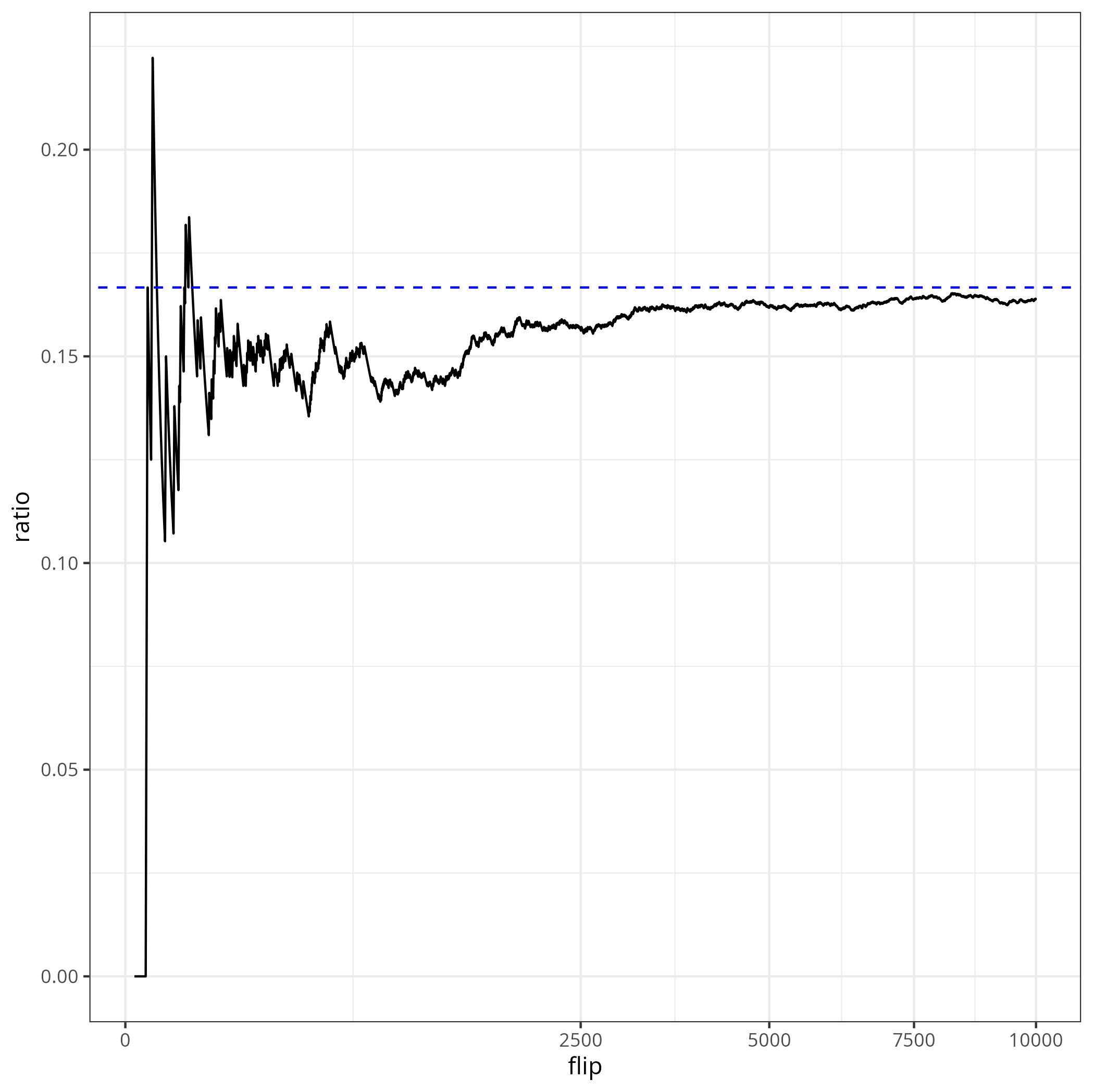
<p>From a quick <a href="/files/posts/03-15-cycle_analysis/consecutive_heads.R">simulation</a> with \(p=1/2\), (flips on the \(x\)-axis, on a square-root scale), it seems like the ratio converges to \(1/6\).
Let us show that analytically.</p>
<div style="text-align: center;">
  <img src="/files/posts/03-15-cycle_analysis/points_timeline.jpg" />
</div>

<h1 id="solution-via-mutual-recursion">Solution via Mutual Recursion</h1>

<p>Consider a (sufficiently large) index \(n\) in our sequence.
The quantity we want to find is the probability that the \(n\)-th coin flip gains one additional point.</p>

<p>There are three possible cases:</p>
<ul>
  <li>the \((n-1)\)-th flip was tails (state T)</li>
  <li>the \((n-1)\)-th flip was heads, and did not gain a point (state H)</li>
  <li>the \((n-1)\)-th flip was heads, and gained a point (state HH)</li>
</ul>

<p>For \(n\) large, the probabilities are <em>stationary</em>, meaning that flipping one more coin does not change their probabilities.
Of course, \(\pi_T\), probability of being in state \(T\), is \((1-p)\), the probability of flipping tails.
Under the stationary distribution, we also have the relations</p>

\[\pi_H = p \pi_T + p \pi_{HH} = p(1-p) + p \pi_{HH}
  \qquad
  \pi_{HH} = p \pi_H\]

<p>The first relation says that the \(H\) state can come from flipping heads from either the \(T\) or \(HH\) states.
The second relation says that to get to the \(HH\) state, we must flip heads from the \(H\) state.</p>

<p>To solve this recurrence, we can unroll:</p>

\[\pi_H = p(1-p) + p^2 \pi_H \implies \pi_H = \frac{p}{1+p}\]

<p>and therefore, \(\pi_{HH} = \frac{p^2}{1+p}\), the solution to our puzzle.
For a fair coin (\(p = 0.5\)), then \(\pi_{HH} = \frac{1}{6}\).</p>

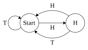
<h2 id="markov-chains">Markov Chains</h2>

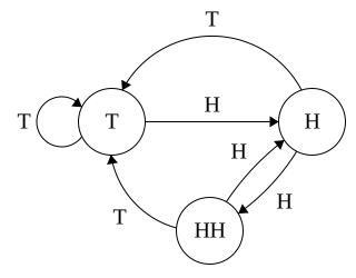
<p>What we have just done is find the stationary distribution of the following Markov Chain:</p>
<div style="text-align: center;">
  <img src="/files/posts/03-15-cycle_analysis/fsm1.svg" alt="Markov Chain using States" />
</div>

<p>The arcs represent the state changes after a coin flip.
We want to find to find the long-term probability of being in the \(HH\) state.</p>

<p>Let \(P(x, y)\) be the probability of transitioning between states \(x\) and \(y\) (zero if there is no arc).
Then, a stationary distribution satisfies the recurrence</p>

\[\pi_y = \sum_x \pi_x P(x, y)\]

<h1 id="towards-a-generalization">Towards a Generalization</h1>

<p>In this problem, we gain points whenever we visit a state.
It is straightforward to generalize to gaining points whenever we visit one of a set of states, by just adding the probabilities!</p>

<p>However, what if we want to gain points instead on an arc?
For example, we can represent this three state markov chain instead using two states, where we get points on the top edge.</p>
<div style="text-align: center;">
  <img src="/files/posts/03-15-cycle_analysis/fsm2.svg" alt="Markov Chain using Edges" />
</div>

<p>As a computer scientist, I care about finite state Markov chains.
For irreducible chains (i.e. corresponding to strongly connected digraphs), there is an alternative way of finding these probabilities.</p>

<h2 id="notation">Notation</h2>

<p>Let us introduce some notation.</p>
<ul>
  <li>\(X_m\), the state of the markov chain after \(m\) steps</li>
  <li>\(P^m(x,y)\) be the probability of moving from state \(x\) to \(y\) in exactly \(m\) steps.</li>
  <li>\(N_n(x,y) = \sum_{m=1}^n 1_{y}(X_m)\), the number of visits to state \(y\) in \(n\) steps, starting at state \(x\).</li>
  <li>\(G_n(x,y) = E(N_n(x,y)) = \sum_{m=1}^n P^m(x,y)\), the expected number of visits to \(y\) from \(x\) in \(n\) steps.</li>
  <li>\(T_{x,y}^r = \min \{ n \ge 1 \mid N_n(x,y) \ge r \}\), the earliest time to hit \(y\) exactly \(r\) times</li>
  <li>\(m_{x,y} = E(T_{x,y}^1)\), the expected time to hit \(y\) starting at state \(x\), i.e. the hitting time</li>
</ul>

<p>For brevity, \(m_y = m_{y,y}, T_y = T_{y,y},\)…</p>

<h2 id="hitting-times-and-stationary-distribution">Hitting Times and Stationary Distribution</h2>

<p>Recall we want to find \(\pi_y\), the stationary distribution of the markov chain.</p>

<p><strong>Theorem:</strong>
<em>The stationary distribution is the reciprocal of the hitting time.</em></p>

\[\pi_y = \frac{1}{m_y} = \lim_{n \to \infty} \frac{N_n(y)}{n}\]

<p><strong>proof:</strong>
First, we show the second equality, that the ratio \(N_n(y, y) / n\) approaches \(1/m_{y}\).
For \(i \ge 1\), we consider \(\omega^i = T_{y}^i - T_{y}^{i-1}\), the marginal time to cycle back to \(y\) for the \(i\)-th time.
Since our transitions are memoryless, then \(\omega^i\) are iid.
Now, by the law of large numbers,</p>

\[\frac{T_{y}^k}{k} = \frac{1}{k} \sum_{i=1}^k \omega^i \to E(\omega) = m_{y}\]

<p>Finally,</p>

\[\frac{T_{y}^{N_n(y)}}{N_n(y)} \le \frac{n}{N_n(y)} \le \frac{T_y^{N_n(y) + 1}}{N_n(y) + 1}\]

<p>where the left and right both converge to \(m_y\).
Thus, \(\frac{n}{N_n(y)}\), and moreover \(\frac{n}{G_n(y)}\), both converge to \(m_y\) as well.</p>

<p>Now, for the first equality, note that for any \(m\), \(\pi_y = \sum_{x \in S} \pi(x) P^{m}(x,y)\).
Therefore, when we sum over \(m\), we have</p>

\[\pi_y = \frac{1}{n} \sum_{m=1}^n \sum_{x \in S} \pi(x) P^m(x,y) = \sum_{x \in S} \pi(x) \frac{G_n(x,y)}{n}\]

<p>Moreover, this holds as \(n \to \infty\), so recalling that \(\sum_x \pi(x) = 1\), then we find that</p>

\[\pi_y = \lim_{n \to \infty} \sum_{x \in S} \frac{G_n(x,y)}{n} \pi(x) = \sum_{x \in S} \pi(x) \frac{1}{m_y} = \frac{1}{m_y}\]

<p>Thus concludes the proof.</p>

<h2 id="computing-hitting-times-using-cycles">Computing Hitting Times using Cycles</h2>

<p>The hitting time \(m_y\) is the expected number of steps starting at \(y\) before reaching \(y\) again.
We can compute this by enumerating all (possibly countable infinite) cycles, computing the probability of taking it, and find the expected length.</p>

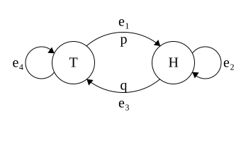
<p>I illustrate this by example.
Consider the following two state Markov chain with states \(T\) and \(H\).
Let \(P(T, H) = p\), \(P(H, T) = q\), and self loops \(1-p\) and \(1-q\) respectively.</p>
<div style="text-align: center;">
  <img src="/files/posts/03-15-cycle_analysis/fsm3.svg" alt="Bernoulli Markov Chain" />
</div>

<p>To find the hitting time (and therefore, the stationary distribution) \(m_T\), then we have the following cycles:
\(e_4\), \(e_1 e_3\), \(e_1 e_2 e_3\), \(e_1 e_2 e_2 e_3\), …</p>

<p>Therefore, we can find the average cycle length, i.e. the hitting time, as</p>

\[\begin{aligned}
m_T &amp; = p(e_4) \cdot 1 + p(e_1 e_3) \cdot 2 + p(e_1 e_2 e_3) \cdot 3 + p(e_1 e_2 e_2 e_3) \cdot 4 + \ldots \\
    &amp; = (1-p) + \sum_{\ell=0}^\infty (\ell + 2) pq (1-q)^\ell \\
    &amp; = (1-p) + 2pq + p(1-q) \sum_{\ell = 0}^\infty (\ell + 2) q(1-q)^{\ell - 1} \\
    &amp; = (1-p) + 2pq + p(1-q) (2 + 1/q) = \frac{p + q}{q}
\end{aligned}\]

<p>Thus, \(\pi_T = \frac{p}{p+q}\).</p>

<p>We can now find \(\pi_H\) in one of several ways.
First, \(\pi_H + \pi_T = 1\), so that \(\pi_H = \frac{p}{p+q}\).</p>

<p>Alternatively, we can note that \(\pi_H / \pi_T\) is the averaged number of times we visit \(H\) in the above cycles.
That is,</p>

\[\begin{aligned}
\frac{\pi_H}{\pi_T} &amp; = p(e_4) \cdot 0 + p(e_1 e_3) \cdot 1 + p(e_1 e_2 e_3) \cdot 2 + \ldots \\
                &amp; = \sum_{\ell=0}^\infty (\ell + 1) pq (1-q)^\ell \\
                &amp; = pq + p(1-q) \sum_{\ell = 0}^\infty (\ell + 1) q(1-q)^{\ell - 1} \\
                &amp; = pq + p(1-q) (1 + 1/q) = \frac{p}{q} 
\end{aligned}\]

<p>so that indeed, \(\pi_H = \frac{p}{q} \frac{q}{p+q} = \frac{p}{p+q}\).</p>

<p>We can summarize this procedure into the following theorem:</p>

<p><strong>Theorem:</strong>
<em>Let \(x\) be any state in a finite irreducible Markov chain, and \(C_x\) be all cycles from \(x\). Then, for any state \(y\),</em></p>

\[\pi_y = \frac{ \text{average visits to } y \text{ in } C_x }{ \text{average length of } C_x }\]

<p>Note that here, we say cycles to allow repeated links, but passing through the start state exactly once.</p>

<p><strong>proof:</strong>
We partition the walk into stages, where each stage is delimited by a cycle in \(C_x\).
Then, \(N_n(y)\) is sum of visits to \(y\) in the \(k\)-th stage.</p>

\[\frac{N_n(y)}{n} = \frac{N_n(y)}{G_n(x) m_x} = \frac{1}{m_x} \frac{N_n(x)}{G_n(x)} \frac{1}{N_n(x)} \sum_{k=1}^{N_n(x)} ( \text{visits to } y \text{ in } k \text{-th cycle} )\]

<p>Now, \(\frac{N_n(x)}{G_n(x)} \to 1\), and \(\frac{1}{N_n(x)} \sum_{k=1}^{N_n(x)} (..)\) approaches the average visits to \(y\) in \(C_x\).
Moreover, the LHS approaches \(\pi_y\), and \(m_x\) is the average length of \(C_x\).</p>

<p>Thus, taking limits, indeed</p>

\[\pi_y = \frac{ \text{average visits to } y \text{ in } C_x }{ \text{average length of } C_x }\]

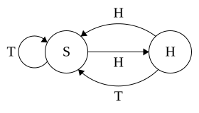
<h1 id="points-on-links">Points on Links</h1>

<p>Let us return to our two-state Markov chain, where we get a point whenever taking the \(H \overset{H}{\to} S\) link.</p>

<div style="text-align: center;">
  <img src="/files/posts/03-15-cycle_analysis/fsm4.svg" alt="Markov Chain using Edges" />
</div>

<p>In general, as we can bisect links into states, then for any start state \(x\),</p>

\[\text{average points} = \frac{ \text{average points in } C_x }{ \text{average length of } C_x }\]

<p>Now, we have the cycles \(T\), \(HT\), and \(HH\) with probabilities \(1-p\), \(p(1-p)\), and \(p^2\) respectively.
The average cycle length is \(1 \cdot (1-p) + 2 \cdot p(1-p) + 2 \cdot p^2 = 1 + p\).
The average points per cycle is \(0 \cdot (1-p) + 0 \cdot p(1-p) + 1 \cdot p^2 = p^2\).
Finally,</p>

\[\text{average points} = \frac{p^2}{1+p}\]

<p>Indeed this is the same solution as via mutual recursion!</p>

<h1 id="concluding-remarks">Concluding Remarks</h1>

<p>Here, we discussed a probability question that could be represented by finding the stationary probability of an irreducible Markov chain.
Then, we described an alternative approach that often leads to smaller Markov chains!</p>

<p>When the underlying digraph is not strongly connected, then this analysis does NOT work.
In particular, the start state now matters.</p>

<p>Addressing this, we need to consider the probability of ending up at each of the strongly connected components.
The general way of handling this is to represent each connected component as an absorbing state, with \(Q\) the new transition probability.
Then, the probability of ending at state \(t\) is</p>

\[Q^0(s,t) + Q^1(s,t) + Q^2(s, t) + \ldots = (1-Q)^{-1}(s, t)\]

<p>where \(\sum_{m=0}^\infty A^m = (1-A)^{-1}\) by Geometric series formula.
\((1-Q)^{-1}\) is called the fundamental matrix.</p>

<p>Apparently, this is a special case of a renewal-reward process.</p>

<h2 id="acknowledgements">Acknowledgements</h2>

<p>The cycle analysis technique was introduced to me by my friend taking CS 438 at UIUC.
Many probablistic networking protocols exhibit simple irreducible behavior which lend themselves nicely to such analysis.</p>]]></content><author><name>Ian Chen</name><email>ianchen3@illinois.edu</email></author><category term="stochastic-processes" /><summary type="html"><![CDATA[Consider an infinitely long sequence of coin flips, i.e. with \(p\) probability heads and \(1-p\) probability tails. You get points for non-overlapping pairs of consecutive heads. How many points do you expect to obtain per flip? That is, what is the limit for the ratio of the number of points over number of flips?]]></summary></entry><entry><title type="html">2026 January Momath Mindbender</title><link href="https://ianchen3.github.io/posts/2026/01/mb" rel="alternate" type="text/html" title="2026 January Momath Mindbender" /><published>2026-01-25T00:00:00+00:00</published><updated>2026-01-25T00:00:00+00:00</updated><id>https://ianchen3.github.io/posts/2026/01/momath</id><content type="html" xml:base="https://ianchen3.github.io/posts/2026/01/mb"><![CDATA[<p>Puzzle from <a href="https://momath.org/mindbenders/">here</a>.
Consider a ladybug starting on the 12-hand of the clock.
During each timestep, it will choose to walk either counterclockwise or clockwise, each with 50% probability.
What is the probability that the last new number it visits is 6?</p>

<p>It will be useful to establish consistent notation.
Let \(p_y\) be the probability that \(y\) is the last new number the ladybug visits.
Let \(X_t\) be the position of the ladybug.
Let \(T_y\) be the first time where \(X_t = y\).</p>

<p>I will also use \(P_x( ... )\) to denote the probability of an event given the starting point of a random walk of \(x\).</p>

<h1 id="gamblers-ruin">Gamblers Ruin</h1>

<p>The first solution I came up with relies on the setup called “Gambler’s Ruin”.
Consider a 1-D symmetric random walk starting at \(0 &lt; x &lt; d\).
I claim that \(P_x(T_d &lt; T_0) = \frac{x}{d}\).</p>

<p>First, observe that \(E(X_t) = x\) (this is called a Martingale process).
This is because at each time step, we make no expected progress towards either endpoint.
Therefore, at time \(T = \min( T_d, T_0)\), then we obtain the equation</p>

\[x = E(X_0) = E(X_T) = 0 P(X_T = 0) + d P(X_T = d) = d P(T_d &lt; T_0)\]

<p>which proves our claim.</p>

<h1 id="solution-one">Solution One</h1>

<p>Now, to solve the puzzle, it remains to enumerate some simple cases.
Consider the sequence in which the ladybug sees new numbers.
Then, in order for 6 to be last, then it must either see 5 before 7 before 6, or 7 before 5 before 6.
That is,</p>

\[p_6 = P_{12}(T_5 &lt; T_7 &lt; T_6) + P_{12}(T_7 &lt; T_5 &lt; T_6)\]

<p>We can decompose</p>

\[P_{12}(T_5 &lt; T_7 &lt; T_6) = P_{12}(T_5 &lt; T_7) \cdot P_5(T_7 &lt; T_6)\]

<p>and</p>

\[P_{12}(T_7 &lt; T_5 &lt; T_6) = P_{12}(T_7 &lt; T_5) \cdot P_7(T_5 &lt; T_6)\]

<p>so that plugging in our expression</p>

\[p_6 = (1/2) \cdot (1/11) + (1/2) \cdot (1/11) = 1/11\]

<h1 id="solution-two">Solution Two</h1>

<p>Following this, I immediately noticed that \(p_1 = p_2 = \ldots = p_{11} = 1/11\).
All the probabilities are uniform!
This hints that there is a simpler explanation.</p>

<p>Indeed, in order for 6 to be the last new number visited, there must be an arc between 5 to 7, or from 7 to 5.
All the steps before reaching either 5 or 7 are superfluous.
Therefore, $p_x = P_5(T_7 &lt; T_6)$.</p>

<p>In words, the probability of seeing 6 last is the probability of starting to one side of 6 and reaching the other side of 6 without hitting 6.
This holds for any starting position.</p>

<p>Now, as there are 11 probabilities, the final step is to show that they sum to 1.
One way of doing this (although there are likely many) is to shift a perspective:
instead of varying the starting point, vary the end point.
As there must be some number that is the last one visited, those probabilities must add to 1.</p>]]></content><author><name>Ian Chen</name><email>ianchen3@illinois.edu</email></author><category term="stochastic-processes" /><category term="puzzle" /><summary type="html"><![CDATA[Puzzle from here. Consider a ladybug starting on the 12-hand of the clock. During each timestep, it will choose to walk either counterclockwise or clockwise, each with 50% probability. What is the probability that the last new number it visits is 6?]]></summary></entry><entry><title type="html">Reinforcement Learning</title><link href="https://ianchen3.github.io/posts/2025/05/rl" rel="alternate" type="text/html" title="Reinforcement Learning" /><published>2025-05-16T00:00:00+00:00</published><updated>2025-05-16T00:00:00+00:00</updated><id>https://ianchen3.github.io/posts/2025/05/rl</id><content type="html" xml:base="https://ianchen3.github.io/posts/2025/05/rl"><![CDATA[<p>Over a year ago now, I took some notes on reinforcement learning from a series of lectures availabe on <a href="https://www.youtube.com/@Mutual_Information">YouTube</a>.
They can be found <a href="/files/2024-summer-rl/Chapter One.html">here</a>.</p>]]></content><author><name>Ian Chen</name><email>ianchen3@illinois.edu</email></author><category term="reinforcement-learning" /><summary type="html"><![CDATA[Over a year ago now, I took some notes on reinforcement learning from a series of lectures availabe on YouTube. They can be found here.]]></summary></entry></feed>